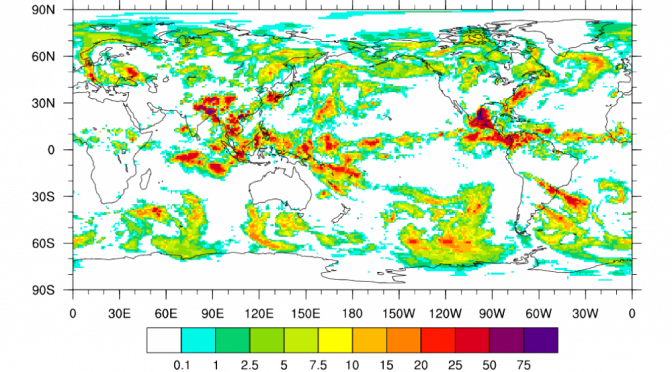
Precipitation Climatology

In the previous two units we discussed how to measure precipitation, the accuracy of precipitation measurements and various methods to interpolate point measurements of precipitation into space. Again we had discussed the accuracy/uncertainty related to these methods. In unit 2, we had already seen the global distribution of precipitation among other global distributions of water cycle relevant quantities. Now that we know how distributions of precipitations are produced we will discuss in this unit various aspects of precipitation climatology. Precipitation climatology is important to assess hydrological events in a watershed, design bridges, potential of agriculture, and water management, among other hydrometeorological aspects. Some concepts like temporal variability, which we discussed within the framework streamflow, are revisited and applied to precipitation. The student may want to repeat reading Dingman’s Chapter 1.9 to 1.9.2.3 (included) once more in preparation of this unit.

Goals

The goal of this unit is to discuss and assess the long-term mean behavior of precipitation, its spatial and temporal variability, extreme events, and human impacts on precipitation.

After successful completion of this unit students will be able to

1. Distinguish between long-term means, spatial and temporal variability, extreme events, and trends in precipitation climatology
2. Calculate precipitation climatology and precipitation accumulation curves from precipitation data
3. Calculate precipitation spatial and temporal variability from precipitation data of an area
4. Discuss precipitation climatology, its variability, trend and extremes in the framework of the water cycle at various scales
5. Produce, analyse, and discuss frequency distributions of extremes, duration
6. Explain the concept of design rainfalls and design floods
7. Determine the probable maximum precipitation in, and the probable maximum flood for a watershed
8. Apply analysis on data consistency (graduate students)

Students’ tasks

1. Read Dingman’s Chapter 4.4 to 4.4.4.3 (included)
2. Download this excel spread sheet of Bering Glacier, Alaska
   1998-2015 precipitation data
3. Fill out the questionnaire and solve the problems in this Unit 6 Application sheet  and submit everything by Thursday 2359 Alaska Time.

Optional reading

We discussed the concepts of temporal variability already in unit 1. Since this concept is revisited here, in preparation of the current unit, the student may want to repeat reading Dingman’s Chapter 1.9 to 1.9.2.3 (included) once more.

You can find more information on human impacts on precipitation in chapter 3.5 of M̦lders, N. 2011, Land-Use and Land-Cover Changes РImpact on Climate and Air Quality, Springer, New York.

FAQ

Q: What is a median of a distribution?

A:  The median of a distribution is the value that separates the higher half of a dataset from the lower half. For instance, 1, 3, 4, 5, 6, 8, 9, 11, 12 has a median of 6.

Q: What is the difference between a mean and median?

A:  The mean is the sum of all values of the dataset divided by the number of data. The median is the  value that separates the higher half of a dataset from the lower half.

Q: What are higher order moments and why are they important in hydrometeorology?

A:  The first monent is the mean. The second moment is the variance of a dataset measures how far the data spread around its mean. It gives the expectation of the squared deviation of a value from its mean.  The standard deviation,   also called sigma σ, is the square root of its variance.  The smaller σ, the narrower the range between the lowest and highest values around the mean. The third moment is  Skewness, which gives the asymmetry of the probability distribution of a real-valued random variable around its mean. At zero skewness, tails on both sides of the mean cancel each other out. It doesn’t say anything about whether the distribution is symmetric or asymmetric. Typically we are interested in whether the distribution is left (negative) or right (positive) skewed.   The fourth moment is  kurtosis, which describes  the shape of a probability distribution. The kurtosis of a univariate normal distribution is 3. When the kurtosis is lower (larger) than 3 fewer and less (more and more) extreme outliers exist than in a normal distribution.

© 2019 Nicole Mölders | All rights reserved